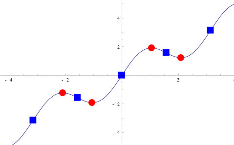
During Geometry optimization we attempt to locate equilibrium structures or Minima . In the general case the Potential Energy Surface (PES) may have several Local Minima and one or several Global Minima (points of the PES with the lowest energy)
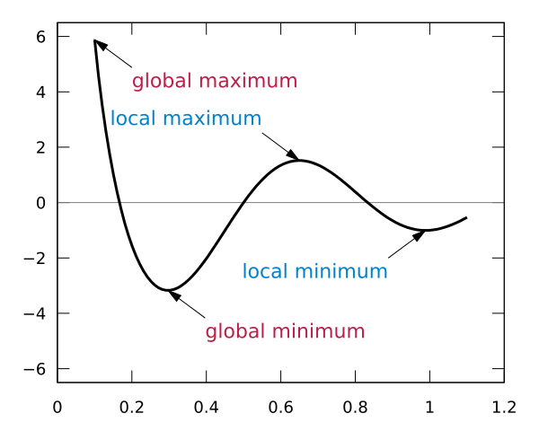 |
| Figure. Local and global minima for a sample function. (From: Wikipedia: Maxima and minima) |
The majority of minimization (optimization) algorithms (including those implemented in a Gaussian program) find the closest minimum (Local or Global) using the gradient descent, i.e. minimization procedure takes steps proportional to the negative of the gradient. The minimization algorithm stops at the point of PES where the gradient is equal (or close ) to zero. This point at the PES is called a Stationary point.
So, in the general case of geometry optimization we can obtain different equilibrium structures if we start from different initial geometries.
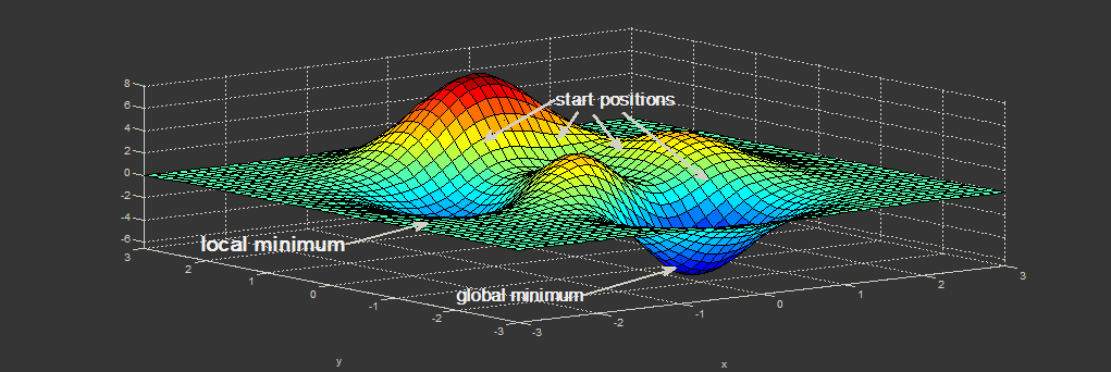 |
| Figure. Minimization problem: depending on the start position (initial geometry), the minimum which is found can either be a local minimum or the global one. (Picture: ©2013.igem.org) |
Also, one needs always to keep in mind that a Stationary point at the PES is defined as a point where the gradient is zero. However, the gradient is zero at both the minima and maxima.
 |
| Figure. The Stationary points are the red circles and they are all relative maxima or relative minima. (From: Wikipedia: Stationary point) |
The nature of Stationery points can be determined by examining the second derivative f''(x) :
To ensure that we obtained an equilibrium structure (or a "true" minimum at the PES) as a result of the geometry optimization in Gaussian we must perform a Frequency Calculation on the optimized geometry. An equilibrium structure should have no negative/imaginary frequencies. A transition state should have one negative/imaginary frequency.
In this tutorial we shall focus on using the Gaussian program for finding the Equilibrium Structures as well as how to distinguish them from the Transition states and Saddle Points via the Frequency Calculations.
Let's perform geometry optimization of an ester
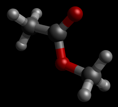 |
| Figure. Initial Geometry of ester. (Picture was generated with Jamberoo and PovRay) |
Its input file for the geometry optimization is here:
# opt rb3lyp/6-311g Title Card Required 0 1 C -1.80660800 -0.53881200 0.00003800 H -2.36857197 -0.26083429 -0.88618435 H -1.65203795 -1.61799553 0.01528765 H -2.37527733 -0.27997817 0.89356445 C 1.91770000 -0.15392600 0.00004700 H 2.46014133 -0.47721892 -0.88594037 H 1.87057918 0.93289423 0.01794681 H 2.37870016 -0.53930211 0.90189718 C -0.48830400 0.17382500 -0.00004900 O -0.31931500 1.39407400 -0.00000900 O 0.56133400 -0.72094200 -0.00006400 |
Opt keyword requests that a geometry optimization be performed.
The resulted output file is here. It looks fine:
Job cpu time: 0 days 0 hours 4 minutes 54.7 seconds. File lengths (MBytes): RWF= 6 Int= 0 D2E= 0 Chk= 2 Scr= 1 Normal termination of Gaussian 09 at Thu Sep 4 16:33:11 2014. |
The optimization is completed and has converged:
Item Value Threshold Converged? Maximum Force 0.000184 0.000450 YES RMS Force 0.000062 0.000300 YES Maximum Displacement 0.000595 0.001800 YES RMS Displacement 0.000204 0.001200 YES Predicted change in Energy=-6.103605D-07 Optimization completed. -- Stationary point found. |
But what is the nature of the obtained stationary point? Is it an equilibrium structure or a saddle point?
To determine the nature of a stationary point we need to perform the frequency calculation. An equilibrium structure has no imaginary frequencies (frequencies which are less than zero). An ordinary transition structure, as a first-order saddle point, is characterized by one imaginary frequency.
Let's modify our initial input file for the geometry optimization and add the Freq keyword to request a frequencies calculation:
# opt freq rb3lyp/6-311g Title Card Required 0 1 C -1.80660800 -0.53881200 0.00003800 H -2.36857197 -0.26083429 -0.88618435 H -1.65203795 -1.61799553 0.01528765 H -2.37527733 -0.27997817 0.89356445 C 1.91770000 -0.15392600 0.00004700 H 2.46014133 -0.47721892 -0.88594037 H 1.87057918 0.93289423 0.01794681 H 2.37870016 -0.53930211 0.90189718 C -0.48830400 0.17382500 -0.00004900 O -0.31931500 1.39407400 -0.00000900 O 0.56133400 -0.72094200 -0.00006400 |
The resulted output file is here. Now it informs us that there is one imaginary frequency:
******    1 imaginary frequencies (negative Signs) ******
Diagonal vibrational polarizability:
      12.4179962       5.9214046      24.7721229
Harmonic frequencies (cm**-1), IR intensities (KM/Mole), Raman scattering
activities (A**4/AMU), depolarization ratios for plane and unpolarized
incident light, reduced masses (AMU), force constants (mDyne/A),
and normal coordinates:
                     1                      2                      3
                     A                      A                      A
Frequencies --    -64.4734                97.8127               190.2938
Red. masses --      1.0666                 1.0645                 3.1290
Frc consts  --      0.0026                 0.0060                 0.0668
IR Inten    --      2.2561                 0.3400                10.7528
 Atom  AN      X      Y      Z        X      Y      Z        X      Y      Z
    1   6     0.00   0.00  -0.02     0.00   0.00   0.02     0.00   0.00   0.17
    2   1     0.25  -0.41  -0.36     0.00  -0.03   0.01    -0.11  -0.17   0.18
    3   1     0.01  -0.02   0.51     0.00   0.00   0.06     0.00  -0.01   0.36
    4   1    -0.27   0.45  -0.31     0.00   0.04   0.01     0.12   0.18   0.19
    5   6     0.00   0.00  -0.03     0.00   0.00   0.03     0.00   0.00   0.20
    6   1    -0.01   0.00  -0.03    -0.18   0.47   0.32     0.33   0.04   0.28
    7   1     0.01   0.00  -0.03     0.18  -0.47   0.32    -0.33  -0.04   0.28
    8   1     0.00   0.00  -0.05     0.00   0.00  -0.54     0.00   0.00   0.41
    9   6     0.00   0.00   0.02     0.00   0.00  -0.01     0.00   0.00  -0.09
   10   8     0.00   0.00   0.05     0.00   0.00  -0.05     0.00   0.00  -0.03
   11   8     0.00   0.00  -0.01     0.00   0.00   0.01     0.00   0.00  -0.29
|
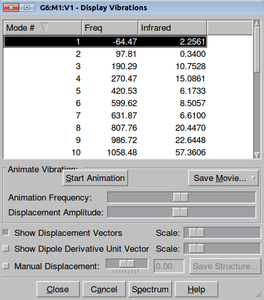
Frequencies also can be quickly inspected after loading output file either into the GaussView or Jamberoo:
 |
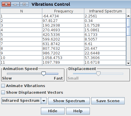 |
| Figure. Frequencies control in GaussView 5 | Figure. Frequencies control in Jamberoo |
Selecting an imaginary frequency we can animate it in both programs as well as visualize the displacement vectors:
 |
| Figure. The vibrations corresponding to the imaginary frequency. It shows that this frequency corresponds to the rotation of Methyl-group around the C-C bond. Generated by GaussView 5.0.9 |
Looking at the animation and displacement vectors we can easily determine that we obtained a transition structure for the rotation of a Methyl-group around the C-C bond.
So, the simplest solution would be in rotating of a Methyl-group around the C-C bond by a few degrees (for example, in GaussView or Jamberoo). Modified input file is below:
# opt freq rb3lyp/6-311g Title Card Required 0 1 C -1.80852300 -0.54070200 0.00068200 H -2.52204418 0.02598931 -0.59766484 H -1.71909218 -1.54887246 -0.39107248 H -2.19697512 -0.57866963 1.01918248 C 1.92070700 -0.14765200 0.00158800 H 2.07150000 0.46363700 -0.88564400 H 2.06599200 0.46348100 0.88984800 H 2.58532900 -1.00358700 0.00369500 C -0.48578600 0.16526800 -0.00194300 O -0.32267200 1.38723900 -0.00010000 O 0.56762900 -0.72330800 -0.00243900 |
The resulted output file is here. So, now there are no imaginary frequencies:
Diagonal vibrational polarizability:
       12.6232142       5.8830575      21.2049024
 Harmonic frequencies (cm**-1), IR intensities (KM/Mole), Raman scattering
 activities (A**4/AMU), depolarization ratios for plane and unpolarized
 incident light, reduced masses (AMU), force constants (mDyne/A),
 and normal coordinates:
                      1                      2                      3
                      A                      A                      A
 Frequencies --     51.8143                98.3061               180.3286
 Red. masses --      1.0744                 1.0825                 2.9795
 Frc consts  --      0.0017                 0.0062                 0.0571
 IR Inten    --      0.9951                 0.2465                11.3694
  Atom  AN      X      Y      Z        X      Y      Z        X      Y      Z
     1   6     0.00   0.00  -0.01     0.00   0.00   0.02     0.00   0.00   0.17
     2   1     0.00   0.00   0.52     0.00   0.00   0.09     0.00   0.00   0.41
     3   1    -0.21   0.45  -0.32    -0.04   0.04  -0.01    -0.22   0.05   0.16
     4   1     0.21  -0.45  -0.32     0.04  -0.04  -0.01     0.22  -0.05   0.16
     5   6     0.00   0.00  -0.01     0.00   0.00   0.03     0.00   0.00   0.20
     6   1     0.00  -0.08  -0.06    -0.17   0.46   0.32     0.32   0.02   0.27
     7   1     0.00   0.08  -0.06     0.18  -0.46   0.32    -0.32  -0.02   0.27
     8   1     0.00   0.00   0.07     0.00   0.00  -0.54     0.00   0.00   0.42
     9   6     0.00   0.00   0.01     0.00   0.00  -0.01     0.00   0.00  -0.09
    10   8     0.00   0.00  -0.04     0.00   0.00  -0.06     0.00   0.00  -0.05
    11   8     0.00   0.00   0.05     0.00   0.00   0.02     0.00   0.00  -0.27
|
It's relatively common problem to get error message like this
GradGradGradGradGradGradGradGradGradGradGradGradGradGradGradGradGradGrad Berny optimization. Using GEDIIS/GDIIS optimizer. Bend failed for angle 16 - 19 - 18 Tors failed for dihedral 9 - 16 - 19 - 18 Tors failed for dihedral 17 - 18 - 19 - 16 Tors failed for dihedral 20 - 18 - 19 - 16 FormBX had a problem. Error termination via Lnk1e in /apps/gaussian/g09d01/g09/l103.exe at Sat Sep 27 20:19:20 2014. |
Inspecting the angle formed by atoms 16, 19 and 18 we see that it has 180 degrees value:
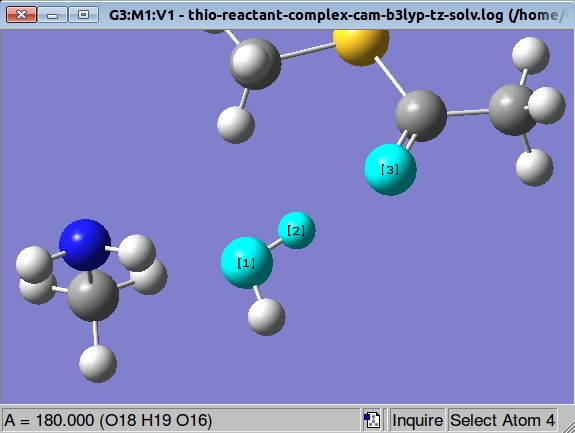
So, what we are going to do is to modify this angle manually and to start over optimization again