
![]() It's a good idea to start to optimize Transition State structure using the inexpensive computational methods, for example, HF/3-21G to get quickly the initial TS which can be used a starting structure for the TS search using more sophisticated methods.
It's a good idea to start to optimize Transition State structure using the inexpensive computational methods, for example, HF/3-21G to get quickly the initial TS which can be used a starting structure for the TS search using more sophisticated methods.
![]() Since Transition State search involves the frequencies calculations it's a good idea to use tighter convergence criteria. To achieve this in Gaussian you can use opt=tight or even opt=verytight.
Since Transition State search involves the frequencies calculations it's a good idea to use tighter convergence criteria. To achieve this in Gaussian you can use opt=tight or even opt=verytight.
![]() Using options opt=tight and especially opt=verytight makes the calculations more computationally expensive, though giving more accurate results.
Using options opt=tight and especially opt=verytight makes the calculations more computationally expensive, though giving more accurate results.
![]() In the case of the DFT methods it's a good idea to use a more accurate numerical integration grid. To achieve this in Gaussian you can use int=fine or int=ultrafine.
In the case of the DFT methods it's a good idea to use a more accurate numerical integration grid. To achieve this in Gaussian you can use int=fine or int=ultrafine.
![]() Using options int=fine or int=ultrafine makes the calculations more computationally expensive, though giving more accurate results.
Using options int=fine or int=ultrafine makes the calculations more computationally expensive, though giving more accurate results.
Now we shall try to locate a Transition State for a double bond migration in CH3CHCH2:

In one of the tutorials devoted to the Potential Energy Scanning we performed a PES for a Hydrogen atom migration from one Carbon atom to another:
Analyzing a structure corresponding to the highest energy during the PES we are not satisfied with the relative position of atoms 1,3,4 and 8:
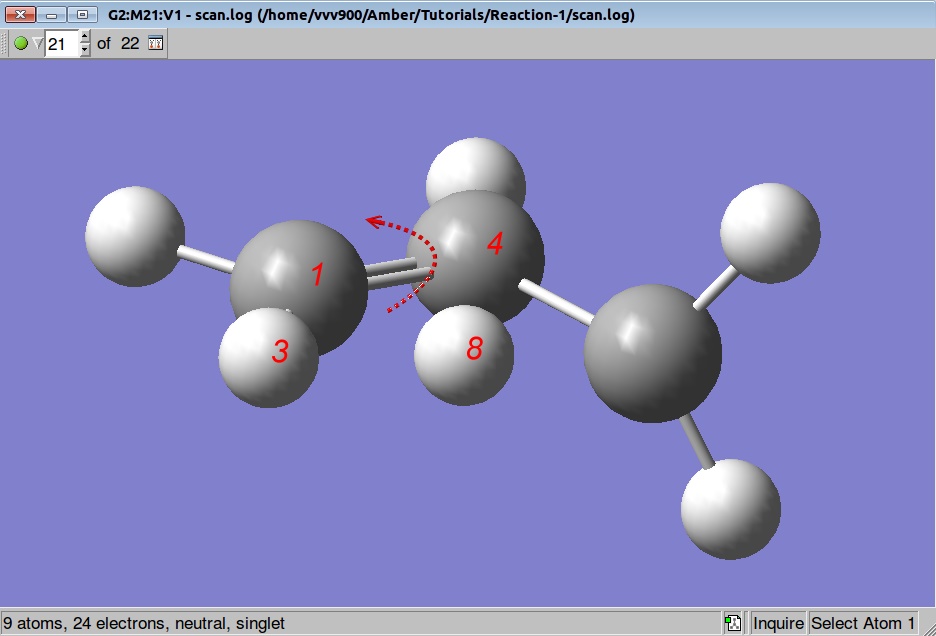
So, before starting the TS search we shall rotate a methylene group by 90 degrees:

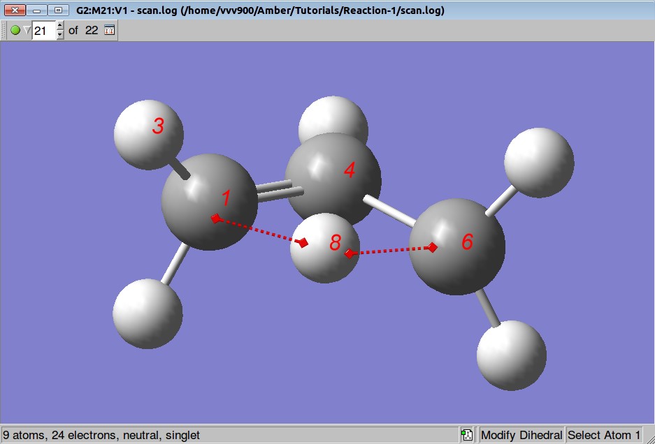
We want to optimize positions of all atoms but to keep distances between atoms C1-H8 and C6-H8 fixed:
The Gaussian input is below:
# opt=(tight,modredundant) freq hf/3-21g Double bond migration: pre-TS optimization 0 1 C -1.02107800 -0.29985000 0.00066800 H -1.35982067 -0.68001024 -0.96440253 H -1.54991113 -0.86429802 0.74553973 C -0.12182800 0.66334900 -0.00182700 H -0.31303900 1.71619300 -0.00129800 C 1.12325000 -0.21853800 0.00055000 H 1.71357900 -0.19828300 0.90365500 H 0.07918200 -0.80218300 0.00371600 H 1.71816300 -0.20065800 -0.89962900 B 1 8 F B 8 6 F |
Modreduntant option tells Gaussian to modify coordinate definition before performing the calculation and it requires a separate input section following the geometry specification.
Lines
B 1 8 F
B 8 6 F
in a Modreduntant section tell Gaussian to keep bonds C1-H8 and C6-H8 fixed (frozen).
Also, we request a frequency calculation on the final optimized geometry (keyword freq).
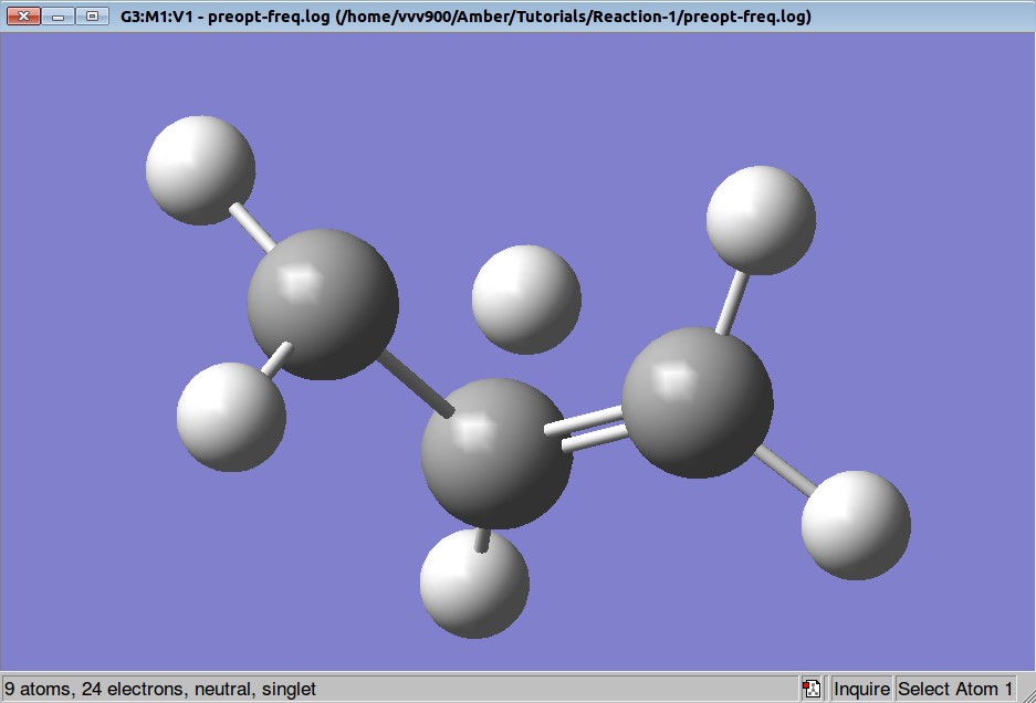
Here is a Gaussian output file and optimized structure (using constrains):
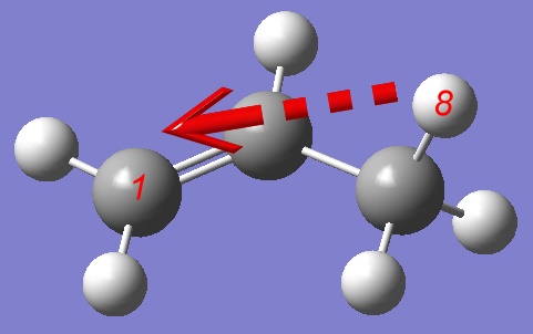
Structure has two negative frequencies
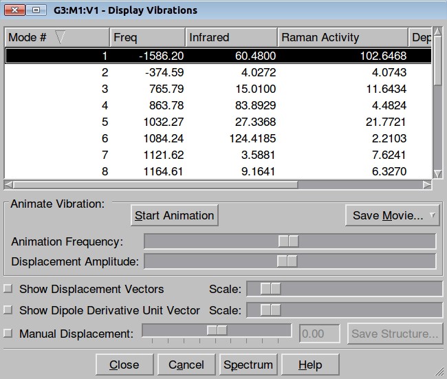
Inspection of the first one suggests that it probably corresponds to the Transition State:
We won't worry about the second negative frequency and prepare an input file for TS location using optimized geometry obtained on the previous step:
# opt=(calcall,tight,ts) rhf/3-21g Transition State calculation 0 1 C 1.01420100 -0.29709000 -0.02717500 H 1.07027900 -1.16773000 0.60444800 H 2.01979200 -0.06814800 -0.37676800 C 0.08859800 0.68216700 0.06776600 H 0.20822000 1.74377500 0.02805100 C -1.08613400 -0.24062400 -0.01268300 H -1.45011200 -0.32884100 -1.02715000 H -0.05978700 -0.84775900 -0.10611600 H -1.88838400 -0.19801700 0.71008500 |
where a keyword TS requests optimization to a Transition State rather than a local minimum, using the Berny algorithm. A keyword calcall specifies that the force constants are to be computed at every point using the current method and that vibrational frequency analysis is automatically done at the converged structure and the results of the calculation are archived as a frequency job.
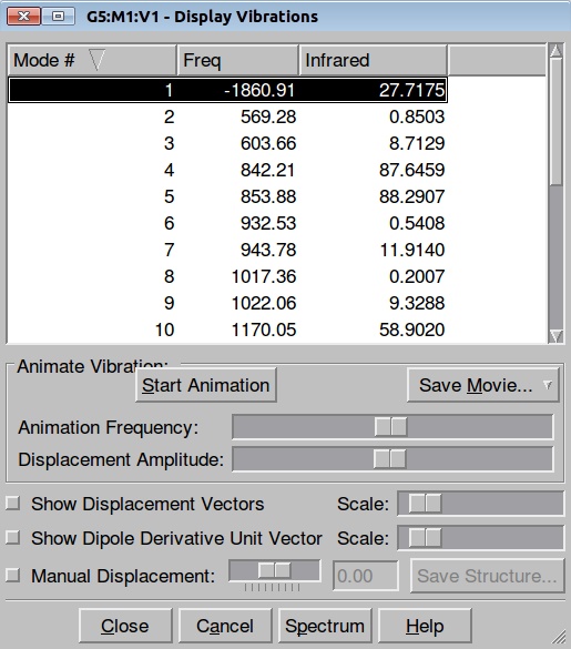
The resulted output file is here. Frequency calculation shows one negative frequency:
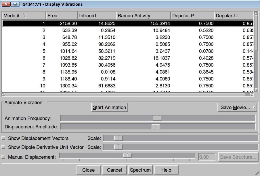
and inspection of the vibration animation ensures that we obtained a "true" Transition State:
Now we can use an obtained TS as a starting structure for a high-level B3LYP method with the correlation consistent basis set, cc-pVDZ:
# opt=(calcall,tight,ts) rb3lyp/cc-pvdz int=ultrafine Transition State calculation Using B3LYP/cc-pVDZ 0 1 C -1.13912400 -0.21831900 0.01485400 H -1.33223100 -0.77367700 -0.88835300 H -2.04696600 0.06309300 0.52856900 C -0.00000100 0.60256100 0.00000100 H -0.00000100 1.67734200 -0.00000200 C 1.13912400 -0.21831800 -0.01485400 H 1.33223700 -0.77367100 0.88835400 H 0.00000000 -1.25172000 0.00000600 H 2.04696300 0.06309000 -0.52857700 |
Here is the resulted output file. Here is a list of frequencies:
Now we can also calculate thermochemistry of the reaction:
|
Energy
|
Enthalpy
|
Free Energy
|
Output File
|
|
| Reagent/Product, in Hartrees |
-117.9116852
|
-117.827546
|
-117.857592
|
|
| Transition State, in Hartrees |
-117.7809058
|
-117.703088
|
-117.731394
|
|
| Reaction thermodynamics,in kcal/mol |
82.07
|
78.10
|
79.19
|